Adaptive compression of periodic signals
or: Pseudo-periodic time series and how to encode them

What do all compression algorithms have in common?
They usually involve some fancy math, but when it comes down to it, their defining tactic is to exploit properties of their input in order to encode the data in fewer bits. Thus a given compression algorithm is typically best applied to a specific type of data. Inversely, given a type of data, the process of selecting an appropriate compression algorithm requires one to precisely identify an exploitable characteristic of the data.
In this article, I’ll introduce a data-compression problem that we faced at Whisker Labs, chart a course through several fields of research, and describe a technique that my colleagues and I developed to address the problem.
An introductory example
Let’s start with a example. Imagine that you’re tasked with building a device which must measure the electrical current going through a 60 Hz AC circuit. The device uses a sensing element to measure current, produces a time series of readings, and then transmits these data to a server for offline processing.
Because alternating current is defined as a sinusoidal function of time, instantaneous measurements are meaningless in isolation. That is to say, since the value of current oscillates periodically, no individual sample will provide a meaningful representation of the dataset as a whole. At best it provides you with a snapshot of the signal’s amplitude at some arbitrary time. To arrive at useful current measurements, you have to capture the full current waveform and then typically compute a quadratic mean to arrive at a numerical result in Amperes.
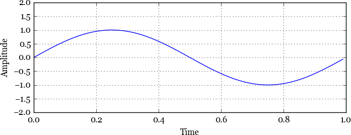 Fig. 1. A single period of a simple sin
wave,
Fig. 1. A single period of a simple sin
wave, y(t) = sin(2πt).
In order to produce data that characterizes the 60 Hz current waveform, the sensor has to sample the circuit at least 120 times per second. In practice, much higher sample rates are required because electrical current can fluctuate on time scales much shorter than one second. Given a sample rate of 1 kHz, if each datapoint is a 16-bit integer, our sensor entails bandwidth of at least 16,000 bits/second or just under 2 kilobytes/second. This may not sound like a lot in the modern era of Big Data™ until one considers the constrained networking environment in which such sensing devices typically operate. For example, an electric utility may deploy these devices on ZigBee networks, which have maximum data rates necessarily measured in kbps. Or the utility may splurge for access to a cellular data network, in which case our sensor’s requirement of almost 40 gigabytes of data per month becomes exorbitantly expensive at any meaningful deployment scale.
So we’ve got ourselves an objective based on a constraint: to reduce the bandwidth utilization of our hypothetical sensor.
Characterizing the data
By definition, data compression involves taking advantage of certain properties of a dataset in order to represent it with fewer bits of information. A simple example is the application of run-length encoding (RLE) to a set of small positive integers, which can result in the elimination of the integers’ leading zeros (in two’s complement).
To apply this strategy to our sensor’s output, we first need to identify patterns in the data and then figure out how we can exploit those patterns. The most ripe characteristic of our dataset has already been mentioned – the fact that AC circuits produce sinusoidal data. For a constant current, the sampled data would form a simple sinusoid (the most basic example thereof is illustrated in Fig. 1). Such a signal could be encoded in only two quantities: the waveform’s amplitude and phase angle. Note that the frequency parameters of the wave equation are fixed for a 60 Hz circuit.
But of course our example is not that simple. As in electric utilities’ use cases, we need to be able to monitor realistic circuits, such as those of a home, commercial building, or data center. These types of circuits entail variable electrical loads, which produce data that are still fundamentally sinusoidal, but are much more messy (see Figure 2).
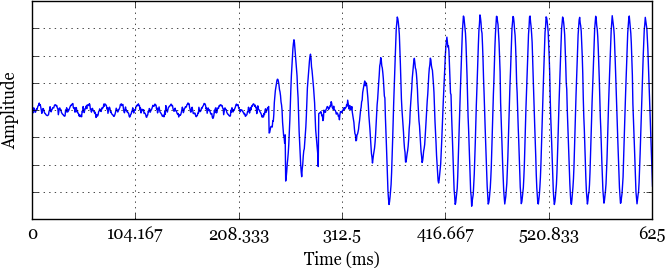 Fig. 2. An example current waveform produced
by a residential electrical load during a state transition. Y axis
units are omitted because the sensor output is technically
unitless. The amplitude is proportional to current, but must go
through a calibration operation to produce measurements in
amps.
Fig. 2. An example current waveform produced
by a residential electrical load during a state transition. Y axis
units are omitted because the sensor output is technically
unitless. The amplitude is proportional to current, but must go
through a calibration operation to produce measurements in
amps.
It turns out that there’s an existing body of research related to signals like these. Whereas vanilla composite waveforms (e.g. Figure 1) are periodic in the sense that they repeat over and over forever, a signal can be termed pseudo-periodic if it can be subdivided into discrete segments of periodicity [2]. An example pointed out in [2] of a pseudo-periodic time series is a heart-beat:
A data set often will exhibit great regularity without exactly repeating. For example, heartbeats always have the characteristic “lub-dub” pattern which occurs again and again, yet each recurrence differs slightly from each other. Some beats are faster, some slower, some are stronger and some weaker. Sometimes a beat may be “skipped”. Nonetheless, the overriding regularity of the heartbeat is its most striking feature.
William A. Sethares, Repitition and Pseudo-periodicity
Interestingly, this property also applies to the audio waveforms of music, leading to applications in compression and rhythm analysis [3]. For the purposes of this article, time series of electrical current measurements also match this definition. This is apparent by visual inspection of Figure 2, wherein the signal can be divided it into three distinct regions:
| Time range | Characteristics |
|---|---|
| 0 - ~220 ms | Low-amplitude, periodic |
| ~220 - ~440 ms | Transient, non-periodic |
| ~440+ ms | High-amplitude, periodic |
Analogously to how one’s heart-rate fluctuates throughout the day during periods of excitement or lethargy, the electrical current going through a circuit fluctuates as connected devices turn on and off. For our hypothetical sensor, this manifests as a mostly-repeating sequence of data, interjected by brief periods of perturbation as the signal shifts to a new pattern.
Leveraging pseudo-periodicity
So we have fancy terminology to describe our data, so what?
Let’s take a step back and consider how a fully periodic time series could be encoded compactly. By definition, the data repeats itself over and over for the duration of the dataset. A variant of run-length encoding could be used, where instead of eliminating sequences of repeated zeros or ones, entire bit sequences would be on the chopping block. Put another way, a periodic dataset presents a similar opportunity to that presented by the collection of positive integers mentioned above, but differs in the cardinality of the repeated pattern.
This principle applies in kind to pseudo-periodic data, provided we can identify subsequences that are sufficiently periodic. Given a time series that can be segmented into locally-periodic regions, we can encode the periodic parts with a single cycle of the data and an integer number of cycles over which the cycle repeats. This would be analogous to deflating a run into a single value and a count in RLE.
This means that for arbitrarily-long sequences of steady-state current readings, all we need to convey is a single 60 Hz cycle’s worth of data and an integer indicating how long the cycle repeats. The efficacy of this technique scales linearly with the duration over which it’s applied – deflating a second’s-worth of steady-state data results in a compression ratio of 60:1, 2 seconds produces 120:1, etc.
Algorithm formulation
In order to make use of this compression technique, we need an automated way to determine that a sequence of data is periodic. This property is often easy to pick out visually, just as the regions of periodicity are apparent in Figure 2. If we divide a periodic region into its constituent cycles and overlay them on top of each other, it’s clear that the cycles have the same shape:
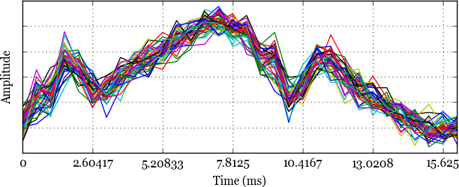 Fig. 3. Forty cycles of electrical current
samples from a region of periodicity overlaid atop each other. The
inter-cycle spread is largely due to random noise imposed by
imperfections in the hardware sensing elements.
Fig. 3. Forty cycles of electrical current
samples from a region of periodicity overlaid atop each other. The
inter-cycle spread is largely due to random noise imposed by
imperfections in the hardware sensing elements.
In order to implement the compression technique described above, an algorithm is needed to detect periodicity. Such an algorithm could be deployed to operate on buffered segments of these time series data, resulting in streaming compression well-suited to sensor output.
Academic interlude
Methods for the detection and characterization of pseudo-periodicity have been a relatively popular sub-field in academic literature since the mid-aughts [5, 6]. The publications we surveyed share an overarching goal of developing an algorithm to determine the precise mathematical description of a signal’s periodic regions. In contrast to our need to simply detect periodicity, the literature was far more general than was our goal. However, there were of course fruitful commonalities, including amplitude mismatch [5] between cycles within a periodic region (which is relevant to any imperfect sensor which measures things in the real world) and the strategy of computing a correlation metric by comparing every ith value in a set of cycles [6].
Quantifying deviance
Rather than diagnosing a signal’s precise parameters and template
function, all we want to do is detect whether or not a time series is
periodic. We could then buffer sensor data for some length of time and
apply our detection function on the buffered windows of data. If the
function returns true, then we know that the window of data can be
reasonably represented as a single cycle, and thus compressed down by
a significant factor.
It is worth noting that our compression technique is lossy. As illustrated by the spread on the y-axis of the lines plotted in Figure 3, cycles’ amplitudes don’t exactly match even in periodic regions. Thus we don’t maintain the full raw data when encoding a long sequence as a single representative cycle. However, in practice we don’t actually lose useful information because the amplitude mismatch can largely be chalked up to minor random noise imposed by imperfections in the sensors’ physical components. In effect, our technique has the added benefit of smoothing the sensor data, if anything.
Our intuition was to apply a standard sum of squares measure of variance to a representative sample of sensor data in order to select a good candidate to serve as the trigger for our algorithm. We first played with a residual sum of squares and ended up choosing root-mean-square deviation because its results are closer in terms of scale to the input data. That is to say, the RSS grows quadratically as variance increases, whereas the RMSD will grow linearly.
With a measure of variance in hand, this leads us into a precise definition of our algorithm.
The algorithm
At a high level, our streaming algorithm will take as input a chunk of buffered time series data, determine whether or not it is periodic, and if so, return a single-cycle representation of the data. Under the hood, we compute the root-mean-square deviation to assess the periodicity of the input.
Given n seconds’ worth of buffered time series data with a known cycle frequency, our “adaptive averaging” algorithm involves three steps:
- Averaging: Compute a cycle average by averaging the corresponding samples of all of the buffered cycles. Put formally, for a set of cycles each comprising m data points, from i = 0 to m compute the average of the ith data points of every cycle.
- RMSD: Taking the cycle average computed in step 1 as the estimator, compute its root-mean-square deviation with respect to the raw cycles themselves.
- Threshold-comparison: Compare the computed RMSD against a predefined threshold to produce a boolean value indicating whether or not the cycle average is sufficiently representative of the data.
The RMSD can be thought of as an error metric for assessing the cycles’ closeness to one another. If this error metric exceeds the threshold, then we cannot reasonably eliminate cycles. If the error metric is lower than the threshold, then we can consider the cycle average to be “close enough” to each raw cycle.
An example is shown in Figure 4. Here we’ve applied the adaptive averaging algorithm with a one-second window size to a sequence of data surrounding that shown in Figure 2. The steady-state cases result in low RMSD values whereas during transient periods of change, the RMSD spikes considerably.
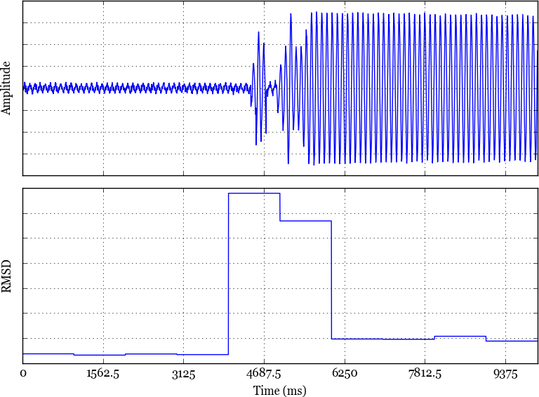 Fig. 4. A ten-second snapshot of
pseudo-periodic time series data and the RMSD values produced by the
adaptive averaging algorithm with a one-second window size.
Fig. 4. A ten-second snapshot of
pseudo-periodic time series data and the RMSD values produced by the
adaptive averaging algorithm with a one-second window size.
Example and results
Bringing this back to our sensor case study, in the steady-state case, we can compress the time series of current measurements down to a cycle average and an integer indicating the number of repetitions that the time series covers. The algorithm is adaptive in the sense that it adapts to the degree of periodicity in the data. This manifests in high compression during steady-state and bursts of lossless data during intervals of change. So we get low data size when current is steady, and then when a fridge or an HVAC system kicks on, we get a brief spike before the current levels off at a new steady-state.
The compression ratio scales linearly with the duration over which data is buffered. The following table shows expected steady-state compression ratios for varying window sizes in terms of the measured quantity’s period, T:
| Window size, in multiples of T | Compression ratio |
|---|---|
| 1 | 1:1 |
| 10 | 10:1 |
| n | n:1 |
Thus, if we were to use a one second window size for our sensor measuring the current of a 60 Hz circuit, we should observe a compression ratio of 60:1 in steady-state cases. Compared to our original bandwith of 16,000 bps, our sensor would emit data at an average rate under 300 bps. This translates to less than one GB/month of total bandwidth, making the aforementioned ZigBee or cellular communication use cases much more feasible.
Other investigated areas of research
Along the way towards coming up with the cycle-averaging + RMSD idea, we investigated a number of areas of research not mentioned thus far. While not as applicable in the end, they made for very interesting reading and drove home the point that there’s more than one way to skin a cat.
From our stream of raw samples, we could feasibly compute a fast
Fourier transform
to decompose the signal into a set of complex numbers or (amplitude,
phase) tuples for each of the harmonics larger than some
threshold. On the server, we could then plug these wave equation
coefficients into sin functions and be done with it. This is a good
option (and one we may eventually implement), but we’ve thus far found
adaptive averaging to be Good Enough for our immediate data size
requirements.
Facebook’s recent paper on their in-memory time series database called Gorilla [1] contains an entire section on time series compression, focusing on delta-of-delta encoding for timestamps and an XOR encoding scheme for values. These weren’t found to be fruitful for our data, particularly because the techniques outlined in the paper rely on the fact that the measurements made by software monitoring systems don’t often fluctuate on small time scales. Our data is much higher-frequency and changes constantly. It was Gorilla’s use of delta-of-delta encoding however that led us down the path of investigating the idea of comparing ith data points across adjacent cycles.
We went down an indulgent path regarding discrete wavelet transforms, a class of functions similar to Fourier transforms that are often used in image compression. At the core of wavelet theory is the notion of decomposing a continuous signal into a discrete series of scaled basis functions. This is compelling, but fell into the same camp as [5] and [6] in seeking a much more complicated outcome than simply detecting a specific property of a time series. Wavelets are a rather impenetrable field of study, but we found [4] to be a reasonable summary.
Conclusion
As we’ve seen, it behooves the bandwidth-concious to be aware of the patterns and properties of their data. By exploiting a property of our specific type of data called pseudo-periodicity, we were able to reduce the average-case size of our real-world sensor data by an order of magnitude.
Update: The compression technique described in this essay has since been deployed fleet-wide at Whisker Labs, resulting in a roughly 84% reduction in bandwidth and overall data size.
@evanm A fun morning: observing an 84% fleet-wide bandwidth reduction due to our adaptive averaging algorithm pic.twitter.com/j26HXUeqYo
— Evan Meagher (@evanm) March 10, 2016
Thanks to Steven Lanzisera, Wilhelm Bierbaum, and Johan Oskarsson for reading and providing feedback on drafts of this essay.
References
- T. Pelkonen, et al, "Gorilla: A Fast, Scalable, In-Memory Time Series Database," Proceedings of the VLDB Endowment, v.8, n.12, p.1816-1827, August 2015. (link)
- W. A. Sethares, "Repitition and Pseudo-periodicity," Tatra Mountains Mathematical Publications, Publication 23, 2001. (link)
- W. A. Sethares and T. W. Staley, "Meter and Periodicity in Musical Performance," Journal of New Music Research, August 2010. (link)
- C. Valens, "A Really Friendly Guide to Wavelets," 1999. (link)
- H. Wong and W. A. Sethares, "Estimation of Pseudo-periodic signals," Dept. of Electrical and Computer Engineering, University of Wisconsin-Madison, May 2004. (link)
- M. Small and J. Zhang, "Detecting and describing pseudo-periodic dynamics from time series," Hong Kong Polytechnic University, August 2007. (link)